Ray is a framework that makes it simple to scale Python applications. The Binomial model is a fundamental technique for options pricing that can benefit significantly from distributed computing.
This post demonstrates how Ray enables you to take existing Python code that runs sequentially and transform it into a distributed application with minimal code changes. While the experiments here were performed on the same machine, Ray also makes it easy to scale your Python code across every major cloud provider.
I'll walk through taking some of these functions and distributing them across multiple processes using Ray, achieving nearly 4x performance improvements.
Binomial Option Pricing Fundamentals
The Binomial model calculates option prices using a tree-like structure that models price movements over discrete time periods. This approach makes several key assumptions:
- The underlying asset has only two possible price movements: up or down
- No dividends are paid during the option's lifetime
- A constant risk-free rate throughout the option's life
- No transaction costs for trading
- Investors are risk-neutral
The model builds its pricing tree using four critical parameters:
uandd: Up and down price movement factorspandq: Risk-neutral probabilities of price movements (wherep+q=1)
Required Model Inputs
The binomial pricing model requires these essential parameters:
S: Current underlying asset priceK: Strike price of the optionT: Time to maturity (in years)r: Risk-free interest ratesigma: Volatility of the underlying assetN: Number of binomial time steps
Python Implementation
The implementation uses standard Python libraries including NumPy and Matplotlib, along with Ray for distributed computing. I'll demonstrate two popular binomial methods: the Cox-Ross-Rubinstein and Jarrow-Rudd approaches.
# Standard Python libraries
import math
import numpy as np
import matplotlib.pyplot as plt
import ray

def Cox_Ross_Rubinstein_Tree (S,K,T,r,sigma,N, Option_type):

    # Underlying price (per share): S;
    # Strike price of the option (per share): K;
    # Time to maturity (years): T;
    # Continuously compounding risk-free interest rate: r;
    # Volatility: sigma;
    # Number of binomial steps: N;

        # The factor by which the price rises (assuming it rises) = u ;
        # The factor by which the price falls (assuming it falls) = d ;
        # The probability of a price rise = pu ;
        # The probability of a price fall = pd ;
        # discount rate = disc ;

    u=math.exp(sigma*math.sqrt(T/N));
    d=math.exp(-sigma*math.sqrt(T/N));
    pu=((math.exp(r*T/N))-d)/(u-d);
    pd=1-pu;
    disc=math.exp(-r*T/N);

    St = [0] * (N+1)
    C = [0] * (N+1)

    St[0]=S*d**N;

    for j in range(1, N+1):
        St[j] = St[j-1] * u/d;

    for j in range(1, N+1):
        if Option_type == 'P':
            C[j] = max(K-St[j],0);
        elif Option_type == 'C':
            C[j] = max(St[j]-K,0);

    for i in range(N, 0, -1):
        for j in range(0, i):
            C[j] = disc*(pu*C[j+1]+pd*C[j]);

    return C[0]

def Jarrow_Rudd_Tree (S,K,T,r,sigma,N, Option_type):

    # Underlying price (per share): S;
    # Strike price of the option (per share): K;
    # Time to maturity (years): T;
    # Continuously compounding risk-free interest rate: r;
    # Volatility: sigma;
    # Steps: N;

        # The factor by which the price rises (assuming it rises) = u ;
        # The factor by which the price falls (assuming it falls) = d ;
        # The probability of a price rise = pu ;
        # The probability of a price fall = pd ;
        # discount rate = disc ;

    u=math.exp((r-(sigma**2/2))*T/N+sigma*math.sqrt(T/N));
    d=math.exp((r-(sigma**2/2))*T/N-sigma*math.sqrt(T/N));
    pu=0.5;
    pd=1-pu;
    disc=math.exp(-r*T/N);

    St = [0] * (N+1)
    C = [0] * (N+1)

    St[0]=S*d**N;

    for j in range(1, N+1):
        St[j] = St[j-1] * u/d;

    for j in range(1, N+1):
        if Option_type == 'P':
            C[j] = max(K-St[j],0);
        elif Option_type == 'C':
            C[j] = max(St[j]-K,0);

    for i in range(N, 0, -1):
        for j in range(0, i):
            C[j] = disc*(pu*C[j+1]+pd*C[j]);

    return C[0]
Performance Comparison: Sequential vs. Distributed
The Ray library transforms your sequential code into a distributed application with minimal changes. Ray provides enterprise-grade features that traditional multiprocessing lacks:
- Multi-machine scaling across cloud providers
- Stateful actors and microservices architecture
- Fault tolerance with graceful handling of machine failures
- Efficient data handling for large objects and numerical computations
Let's compare the performance difference between sequential execution and Ray's distributed approach.
Sequential Execution
First, let's establish our baseline with sequential processing. This approach calculates option prices for different step counts using standard Python loops:
def generate_options_price_steps(
S=100,
K=110,
T=2.221918,
r=5,
sigma=30,
PC : Literal["C", "P"] = 'C'
):
"""
Generate option pricing data across different step counts
"""
r_float = r/100
sigma_float = sigma/100
# Test with step counts from 50 to 5000
runs = list(range(50,5000,50))
CRR = [Cox_Ross_Rubinstein_Tree(S, K, T, r_float, sigma_float, i, PC) for i in runs]
JR = [Jarrow_Rudd_Tree(S, K, T, r_float, sigma_float, i, PC) for i in runs]
return runs, CRR, JR
def run_local(PC : Literal["C", "P"] = 'C'):
"""Execute sequential option pricing"""
start_time = time.time()
runs, CRR, JR = generate_options_price_steps(PC=PC)
plt.plot(runs, CRR, label='Cox_Ross_Rubinstein')
plt.plot(runs, JR, label='Jarrow_Rudd')
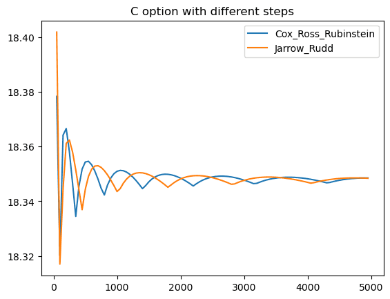
plt.title(f'{PC} option with different steps')
plt.legend(loc='upper right')
plt.show()
duration = time.time() - start_time
print(f'Local execution time: {duration}')run_local("P")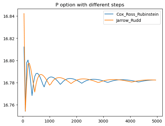
Put option sequential execution time: 131.55 seconds

Call option sequential execution time: 128.26 seconds
Distributed Execution with Ray
Ray transforms sequential Python code into distributed applications with minimal modifications. The key advantage is that you don't need to rewrite your existing code from scratch-Ray handles the complexity of distributed computing for you.
Modern applications require capabilities that traditional modules like multiprocessing can't provide:
- Multi-machine execution across cloud infrastructure
- Stateful microservices with inter-service communication
- Fault tolerance for handling machine failures and preemption
- Optimized data handling for large objects and numerical computations
Ray addresses these requirements by converting functions and classes into tasks and actors in a distributed environment. Here's how to transform our sequential code:
The transformation requires only two key changes: adding the @ray.remote decorator and using ray.get() to collect results:
# Convert functions to Ray tasks with a single decorator
@ray.remote
def Cox_Ross_Rubinstein_Tree_distributed(S,K,T,r,sigma,N, Option_type):
    # Identical implementation to sequential version
    return C[0]

@ray.remote
def Jarrow_Rudd_Tree_distributed(S,K,T,r,sigma,N, Option_type):
    # Identical implementation to sequential version
    return C[0]

def generate_options_price_steps_remote(
    S=100,
    K=110,
    T=2.221918,
    r=5,
    sigma=30,
    PC : Literal["C", "P"] = 'C'
):
    """
    Generate distributed option pricing data across different step counts
    """
    r_float = r/100
    sigma_float = sigma/100

    # Same test range as sequential version
    runs = list(range(50,5000,50))

    # Execute tasks in parallel and collect results
    CRR = ray.get([Cox_Ross_Rubinstein_Tree_distributed.remote(S, K, T, r_float, sigma_float, i, PC) for i in runs])
    JR =  ray.get([Jarrow_Rudd_Tree_distributed.remote(S, K, T, r_float, sigma_float, i, PC) for i in runs])

    return runs, CRR, JR

def run_remote(PC : Literal["C", "P"] = 'C'):
    """Execute distributed option pricing"""
    start_time = time.time()

    # Initialize Ray cluster
    ray.shutdown()  # Clean shutdown if already running
    ray.init()      # Start Ray

    runs, CRR, JR = generate_options_price_steps_remote(PC=PC)
    plt.plot(runs, CRR, label='Cox_Ross_Rubinstein')
    plt.plot(runs, JR, label='Jarrow_Rudd')
    plt.title(f'{PC} option with different steps')
    plt.legend(loc='upper right')
    plt.show()
    duration = time.time() - start_time
print(f'Remote execution time: {duration}')run_remote("P")
Put option distributed execution time: 31.53 seconds
Call option distributed execution time: 33.93 seconds
Performance Results
The results demonstrate Ray's dramatic performance improvement:
- Put options: 131.55s → 31.53s (4.17x speedup)
- Call options: 128.26s → 33.93s (3.78x speedup)
This nearly 4x performance gain comes from Ray's ability to distribute computational tasks across multiple CPU cores with minimal code changes. The same algorithms that took over two minutes sequentially now complete in under 35 seconds.
Ray makes it straightforward to transform sequential Python code into distributed applications, providing enterprise-grade scalability without requiring a complete rewrite of your existing codebase.
References
- YuChenAmberLu: Options Calculator with Binomial model Notebook
- Ray Team: Ray Documentation
- Personal Notes: Ray Core Remote Functions